Stereo vision with the use of a Virtual Plane in the space
Bernard COUAPEL (KE Baïnian)
http://www.multimania.com/merciber/paper1/paper1.html
ENSA / IRISA Rennes (France).Institute of Information Science, Northern Jiaotong University Beijing (China).
Published in the Chinese Journal of Electronics Vol.4 N°2, April 1995
This paper presents a geometrical method to calculate the position of points in 3D space from two different views. Our method is divided into two steps. The first step is two-dimensional and defines the epipolar geometry. It calculates a double projection of the homologous image on the reference image through a Virtual Intermediate Plane. We use eight corresponding points to calculate the transformation of the homologous image. The disparity between the corresponding points in a same referential allows us to get some information about the position of the 3D points. The second step calculates the coordinates of points in a projective space. The calculation of 3D coordinates consists of a simple transformation of projective to cartesian coordinates with 5 points in the case of a pinhole camera, and 4 points for the parallel projection. The aim of our method is to calculate the relative positionning without any knowledge on 3D coordinates of points, to offer controls along the calculation and to postpone use of the reference pointuntil the end of the calculation.
Keywords: stereovision, geometry, calibration, relative positionning
One major subject of research in computer vision is the stereovision i.e. the calculation of points in the space, using their images on different viewing positions by a pinhole camera. The conventional approach is based on camera calibration which implies to calculate the parameters of the cameras and their relative positioning. Some work using this approach can be found in [CHAU89] and [FAN_91]. This has also been the method of calculation used in photogrametry for many years [CARR71] [HURA60]. A recent approach was initiated by [LONG81] who presented a method to calculate the epipolar geometry that is infered by the pinhole model of camera. This work has been extended in 3D by algebraic methods which recover the camera transformation matrices with the use of five points of the scene [FAUG92] [LUON92], and with geometric methods which use two sets of four coplanar points in the scene [MORI93] [MOHR92]. Recently [SHAS93] has proposed a method of reconstruction using four points in the scene defining a tetrahedron and the center of projection of the camera as a fifth reference point. The author recovers a projective invariant and defines a new stuctural description: the projective depth.
Our approach differs from [SHAS93] in the way that we calculate the projective depth. We use a Virtual Intermediate Plane (VIP) which is defined by three known points of the scene . We recover the projective depth by a double projection of a point on the homologous image on the reference image through the VIP.
The first step of our method is described in section 3 of this paper. It calculates the epipole and the transformation of the homologous image towards the reference one with the use of 8 corresponding points. The second step presented in section 4 calculates the relative positionning of the points in a projective referential made of 5 known points. The cartesian coordinates are obtained at the end of the algorithm by a simple tranformation projective / Cartesian space, with the use of the coordinates of five points in the case of a pinhole model, and four points in the case of parallel projection.
The advantage of our method is that the first step gives controls on the validity of the corresponding points, and that the 2D transformation of the homologous image gives informations on the 3D position of points. This transformation is also useful for the global matching of the two images, because if one facet of the 3D object maps the VIP, then the corresponding parts in the images are directly matched.
The cartesian coordinates are noted in lower case and the projective coordinates in upper case. For all the points described below, we give the Cartesian and the projective coordinates.
We use two cameras S and S' and the homologous of an element x for S is noted x' on S'.
For the system S, the image plane is noted Q, the projection center: C (xc,yc,zc) or (Xc,Yc,Zc,Tc), the epipole: E (xe,ye) or (Xe,Ye,Ze), and the image points: Mi (xi,yi) or (Xi,Yi,Zi).
The 3D points are noted Pi (xi*,yi*,zi*) or (Xi*,Yi*,Zi*,Ti*).
We also use a Virtual Plane in the space which is noted VIP. The points on the VIP are noted in lower case.
The two homographies corresponding to the projection of Q on VIP through C and the projection of Q' on VIP through C' are noted respectively H1 and H2.
The recalculation of a point Mi' from Q' to Q with the VIP method is noted Mi" (xi",yi") or (Xi",Yi",Zi").
We work on a pair of stereoscopic images. One is called the reference image. It remains unchanged during the calculation and corresponds to the plane Q of the system S. The other one is called the homologous image. It is transformed during the calculation and corresponds to the Q' plane of the system S'.
The relation between the 3D points and their image on the projection plane is presented in Fig.1. We see that the 5 points P1,C,C',M1 and M1' belong to the same plane in the space and define the epipolar geometry [LONG81] which describes two sets of lines that cross on the intersection of the two image planes. The homologous lines are called epipolar lines and the centers of the pencils the epipoles. The epipoles correspond to the intersection of the line defined by the projection centers with the image planes. This geometry leads to constraints which will use in this article.

Fig.1: Epipolar geometry
Fig.2 shows a simple case of stereo vision in which the two projection planes belong to the same plane defined by three points (not aligned). In this case there is only one epipole e.

Fig.2: simplified stereovision
The calculation of the point P is easily done by crossing the lines {C,M} and
{C',M'} in the space.
If the positions of C and C' are unknown, we can calculate them with the use
of two points P1 and P2, and their images (M1,M1') (M2,M2') on Q. C is defined
by the intersection of {P1,M1} and {P2,M2} and C' by the intersection of {P1,M1'}
and {P2,M2'}. We have used three points to define Q and 2 points to calculate
the projection centers.
Our goal is to bring the general case of stereovision to this particular case.
The usual problem of stereovision is presented in fig.3. The two projection planes are situated anywhere in the space but the pinhole model infers an epipolar geometry. All the points of the figure 3 belong to the same plane.
We bring this case of stereo vision to the particular case described in the beginning of this section by a method which will use a Virtual Intermediate Plane (V.I.P.) in the space.

Fig.3: General case of stereovision
This method is divided into two steps:
The first one is two-dimensional. It defines the composition H of the projection H2 of Q' on the VIP through C', and the projection H1-1 of the VIP on Q through C. If we consider the images of a 3D point P, the result of the calculation of its image M' on Q' is the point M" on Q, which corresponds to the composition H of the two projections. The characteristics of the relation are that if the 3D point P belongs to the VIP, then the points M and M" are fused, and if P does not belong to the VIP, then M and M" are aligned with the epipole E on Q (epipolar geometry). The solution is calculated with 8 corresponding points on the two images.
The second step consists of projecting Q and H(Q') on the VIP, and calculating the position of C and C' in the space. Thus, we bring the general case of stereovision to the simplified case described at the beginning of this section. The calculation uses the coordinates of 5 non coplanar 3D points and their images. But as we can consider these 3D points as a projective referential, it is possible to calculate the coordinates in a projective space, and to obtain the relative positioning of all the points in the scene without the use of 3D coordinates.
The projections H1 of Q on the VIP through C and the projection H2 of Q' on the VIP through C' are homographies from plane to plane.
Properties of the homographies [EFIM81]:
- a non degenerated homography is a bijective application defined by an inversible matrix.
- the homographies form a group, so a composition of homographies, or the inverse of an homography are also homographies.
- an homography preserves the cross ratio of four aligned points.
We calculate the composition H of the projections H2 and H1-1 which transform the points Mi' on Q' to the points Mi" on Q. This composition is an homography with the following properties:
1) The transformed images Mi"=H(Mi') of the points Pi which belong to the VIP map the points Mi on Q.
2) The transformed images Mi"=H(Mi') of the points Pi which are not on the VIP belong to the line {Mi,E} on Q.
We choose a projective referential on each plane made of three pairs of corresponding points (M1,M2,M3 / M1',M2',M3'), i.e. images of the same point in the space, and an arbitrary unity point, for example the center of gravity of each triplet of points. These triplets are called basic points. The 3D points corresponding to these basic points define the virtual plane in the space. The (xi,yi) Cartesian coordinates on Q are transformed into (Xi,Yi,Zi) projective coordinates by the matrix:
|
|Xi| |x1 x2 x3|-1 |xi| |
Tranformation into projective coordinates
We built a similar matrix for Q', with the coordinates of the homologous points.
So the points (M1,M2,M3) on Q and (M1',M2',M3') on Q' have the projective coordinates:
M1 (0,0,1), M2 (0,1,0) M3 (1,0,0)
M1'(0,0,1), M2'(0,1,0) M3'(1,0,0)
First property of H:
The transformed images Mi"=H(Mi') of the points Pi which belong to the VIP map the points Mi on Q.
H(M1') = M1, H(M2')=M2, H(M3')=M3
H(0,0,1)=(0,0,1), H(0,1,0)=(0,1,0), H(1,0,0)=(1,0,0)
Thus the homography is reduced to the matrix:
|
| a 0 0 | |
with a.b.c different from 0.
All the points on Q and Q' are transformed in projective coordinates with their respective matrix.
Second property of H:
The transformed images Mi"=H(Mi') of the points Pi which are not on the VIP belong to the line {Mi,E} on Q. These points are called secondary points. The alignment of the points {Mi,Mi',E} with the epipole (Xe,Ye,Ze) leads to the following system of equations:
|
|Xi a.Xi' Xe| |
Equ.1: Alignment of homologous points with the epipole
Or:
|
Xe[c.Yi.Zi'- b.Zi.Yi'] - Ye[c.Xi.Zi' - a.Zi.Xi'] + Ze[b.Xi.Yi' - a.Yi.Xi'] = 0 |
We eliminate the coordinates of E, in order to obtain a better stability. For each equation, we take three secondary corresponding points with indices i,j,k (different from each other, and superior to 3 to avoid working with basic points that are fused by definition). The new system of equation is now:
|
|c.Yi.Zi'-b.Yi'.Zi a.Zi.Xi'-c.Zi'.Xi b.Xi.Yi'-a.Xi'.Yi| |
Equ.2: System of equations to calculate the homography
With n points, we can build C(n,3) equations of this kind, that correspond to a system of equations with the bounded unknowns a, b, c:
|
A.b/c + A'.c/b + B.c/a + B'.a/c + C.a/b + C'.b/a + D = 0 |
Equ.3: Form of the equation to calculate the homography
In which the bounded unknowns can be written
xa=b/c, xa'=c/b, xb=c/a, xb'=a/c, xc=a/b, xc'=b/a, so:
|
A.xa + A'.xa' + B.xb + B'.xb' + C.xc + C'.xc' + D = 0 |
Linear system of equation with six unknowns
With x1.x1' = x2.x2' = x3.x3' = 1
We find a least squares solution to this system of equation, and we obtain two
controls of the solution:
- The least squares error LSQ of the system with C(n,3) equations and 8 unknowns.
- The error of coherence on the bounded variables which must respect the constraint
x1.x1' = x2.x2' = x3.x3' = 1, noted ERRCOEF.
We calculate a solution with 8 corresponding points, 3 corresponding basic points
which define the VIP and 5 corresponding secondary points which build C(5,3)
= 10 linear equations
As the coefficients a,b,c are up to a factor, we can set c=1. We obtain the
coefficients a, b and the controls described before. We can calculate the epipoles
E and E'which have the same projective coordinates with the equation 1.
This solution allows us to recalculate the homologous image Q' and superpose
it with the reference image Q. The corresponding basic points are fused and
the corresponding secondary points aligned with the epipole. All the images
Mi,Mi" of the points Pi belonging to the VIP are fused, and the other aligned
with the epipole. The homologous epipolar lines are superposed, so we have solved
the problem of epipolar geometry. We do not need to know the position of the
VIP in the space in this step.
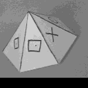
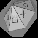
We have used our method on different kinds of images and here we present an example of solution with two images of a pyramid. The basic points (i.e. the VIP) are chosen on the base of the pyramid, and we can observe the transformation of the homologous image with the calculated homography. All the points of the basis of the pyramid are fused and the disparity between the other corresponding points which depend on the distance of the 3D point from the VIP, and the distance from the camera. We also show the influence of the basic points on the transformation of the homologous image. In each case, the basic points form the vertices of the triangle drawn on the superposition of the reference image (which does not change) and the transformed homologous image.
|
|
|
 Transformed homologous image (3) |
 Superposition of (1) and (3) |
 |
|
 |
|
|
 |
 |
|
|
 |
 |
|
 |
 |
|
Reference image (1)
|
Transf.homol.image(2)
|
Superposition of (1) and (2)
|
Example of four different tranformations along with different basic points
All the elements that we use for this second step of the processing are presented in fig. 4. We use the coordinates of five non coplanar points Pi in the space and their images Mi and Mi" on the image plane Q.

Fig.4: Alignment of points in the space
In order to bring the problem of stereovision to the simplified one presented
in section 2 of this article, we have to project the image plane Q on the VIP
and to calculate the coordinates of the projection centers C and C'.
We use the images {M1,M2,M3} and {M1',M2',M3'} of the 3D points {P1,P2,P3} as
a projective referential on Q and Q' with the center of gravity of the three
points as the unity point of each projective referential, like in the previous
section. As we calculate the homography H between Q' and Q corresponding to
the double projection through the VIP, we are able to transform the coordinates
on Q' into H(Q') coordinates on Q. Thus we have only the plane Q to project
through C on the VIP.
If we consider the points {P1,P2,P3,P4,P5} like a projective referential R of
the space, then the projective coordinates of points are:
P1 (1,0,0,0), P2 (0,1,0,0) P3 (0,0,1,0) P4 (0,0,0,1) P5(1,1,1,1) and a point
Pi in R has the coordinates Pi(Xi,Yi,Zi,Ti).
The VIP is defined by the three points (P1,P2,P3). Thus the equation of this
plane is T=0 and the projection H1 of Q on the VIP is defined by an homography
with two parameters u and v like for Q and Q'. We also need to calculate the
coordinates of the projection centers which we can write as C: (Xc,Yc,Zc,1)
and C': (Xc',Yc',Zc',1). So we have a total of 8 unknowns to calculate in order
to define the projection of Q on the VIP and the projective coordinates of C
and C' in the referential R.
The H1 projections of {M1,M2,M3,M4,M5} and {M1",M2",M3",M4",M5"} on the VIP
have the coordinates m1=m1"(1,0,0,0), m2=m2"(0,1,0,0), m3=m3"(0,0,1,0), m4(u.x4,v.y4,z4,0),
m4"(u.x4",v.y4",z4",0), m5(u.x5,v.y5,z5,0), m5"(u.x5",v.y5",z5",0) in R.
We consider the alignment of the points (m4,P4,C), (m4",P4,C'), (m5,P5,C) and
(m5",P5,C'). Each line in the projective space R can be defined by the intersection
of two planes, and leads to 2 equations.
So we have a linear system of 8 equations with 8 unknowns that gives us a unique
solution, i.e. the projection H1 of Q through C on VIP and the projective coordinates
of C and C'.
Now, we have asimple way to calculate the projective coordinates of an unknown
3D point P with the use of the projective coordinates of its two images M and
M" on Q. First we transform the projective coordinates M and M" on Q into coordinates
on the VIP m=H1(M), m"=H1(M"). Then we calculate the intersection of the lines
(C,m) and (C',m") in the projective space R. The result is the projective coordinates
of P in R. The calculation of the cartesian coordinates is done by applying
the (4x4) projective -> cartesian matrix on the projective coordinates of
P.
We have brought the general problem of stereo vision down to the simplified
one presented in section 2. We are able to calculate the relative positionning
of the points in a projective space if we don't know the 3D coordinates of the
5 points that form the projective referential, and we calculate the Cartesian
coordinates if we know the position of these points in the space. The use of
the 3D coordinates is postponed at the end of the calculation. This avoids the
propagation of errors on the approximation of the reference points in the space.
The parallel projection is a simplified model of the pinhole model because the projection centers and the epipoles are situated at infinity. So we have only to calculate the directions of the projections on Q and Q'. Thus we need only four non coplanar points to solve the problem. The position of an unknown point P in the space is obtained by the intersection of the two parallels to (m4,P4) and (m4",P4) passing respectively by m and m', as shown in fig. 5.

Fig.5 Relations in the space with the parallel projection
In this particular case, we don't need to use the double projection, we simply convert the image coordinates into barycentric coordinates related to the referential {M1,M2,M3} for Q and {M1',M2',M3'} for Q' then we convert them to Cartesian coordinates related to the referential {P1,P2,P3} on the VIP.
|
|x| |x1 x2 x3| |X| |
Transformation into barycentric coordinates
Solution
1) Transformation of the coordinates into barycentric coordinates for the points
Mi on Q with the referential {M1,M2,M3}, and for the points Mi' on Q' with the
referential {M1',M2',M3'}.
2) Tranformation of the barycentric coordinates of the points Mi and Mi' into
mi and mi' Cartesian coordinates on the VIP in relation to the referential {P1,P2,P3,P4}.
The 3D point P4 and its images on the VIP are known. So (m4,P4) and (m4',P4)
define the two directions of the parallel projections.
3) Any point P is calculated by the intersection of the parallels to (m4,P4)
and (m4',P4) passing respectively by m and m'.
We have tested the two methods of calculation on several objects and here we present some results on the pyramid object. We have three kinds of errors in the evaluation of the points :
1) The camera is not a real pinhole model and there are some distortions on the image plane.
2) The position of the corresponding points on the images may have an error of one to three pixels from the real points.
3) The 3D points have been measured with a ruler and may also have some errors of approximation.
The aim of this experimentation is not to get the best accuracy but to evaluate the interest of our method for a normal use.
The depth of the object is about 10 cm and the distance camera - object is about one meter. Table 1 shows the positions of the points measured on the images (X,Y), (X',Y') and on the object (X3D,Y3D,Z3D).
|
X |
Y |
X' |
Y' |
X3D |
Y3D |
Z3D |
|
15 |
150 |
89 |
41 |
0 |
0 |
0 |
|
454 |
106 |
395 |
186 |
5 |
8.8 |
0 |
|
343 |
188 |
169 |
202 |
7.5 |
4.4 |
0 |
|
164 |
34 |
255 |
26 |
2.5 |
4.4 |
5 |
|
93 |
128 |
121 |
61 |
2.5 |
1.1 |
1.9 |
|
306 |
100 |
272 |
126 |
4.8 |
5.8 |
2.1 |
|
336 |
50 |
457 |
97 |
0 |
8.8 |
0 |
|
112 |
213 |
16 |
124 |
5 |
0 |
0 |
|
206 |
133 |
157 |
111 |
4.7 |
3.2 |
2 |
|
312 |
58 |
370 |
96 |
2.1 |
7.2 |
1.9 |
Table 1: Coordordinates of the points on the images and on the object
The first step which calculates the double projection through the VIP gives the results:
Homography resulting from the two projections: a=0.997 b=0.986 c=1 LSQ=0 ERRCOEF=0.03
Position of the epipoles on Q and Q': E=(1860, -1177) E'=(1573, -922)
The least squares error LSQ and the error on the bounded variables ERRCOEF are small and show that the 2D solution is good. So we can apply the second part of our method of calculation.
The next two tables show the results of the 3D calculation with the pinhole model and the parallel projection. Each line of the table shows the position of one point (Xreal,Yreal,Zreal) measured on the object (corresponding to the table 1), the calculated point in 3D (Xcalc,Ycalc,Zcalc), the least squares error LSQ for the intersection of the two line in the space (4 equations and 3 variables) and the distance between the 3D measured point and the calculated one.
|
Xreal |
Yreal |
Zreal |
Xcalc |
Ycalc |
Zcalc |
LSQ |
dist. |
|
0.00 |
0.00 |
0.00 |
0.00 |
0.00 |
0.00 |
0.00 |
0.00 |
|
5.00 |
8.80 |
0.00 |
5.00 |
8.80 |
0.00 |
0.00 |
0.00 |
|
7.50 |
4.40 |
0.00 |
7.50 |
4.40 |
0.00 |
0.00 |
0.00 |
|
2.10 |
7.20 |
1.90 |
2.10 |
7.20 |
1.90 |
0.00 |
0.00 |
|
2.50 |
4.40 |
5.00 |
2.50 |
4.40 |
5.00 |
0.00 |
0.00 |
|
2.50 |
1.10 |
1.90 |
2.52 |
1.53 |
1.82 |
18.21 |
0.44 |
|
4.80 |
5.80 |
2.10 |
4.90 |
5.70 |
2.17 |
17.08 |
0.16 |
|
0.00 |
8.80 |
0.00 |
-0.94 |
8.72 |
-0.29 |
1.07 |
0.99 |
|
5.00 |
0.00 |
0.00 |
4.42 |
0.12 |
-0.48 |
3.61 |
0.76 |
|
4.70 |
3.20 |
2.00 |
5.00 |
3.17 |
2.07 |
41.42 |
0.31 |
Table 2: Results of the calculation with the pinhole model
Homography between the reference image Q and the VIP: u=0.0174 v=0.0183 w=0.017
Position of the projection centers: C=(50,5, -5.9, 37.9) C'=(79.9, 26.3, 80.7)
Total distance between the measured points and the calculated points: 2.6 cm, which represents a mean error of 2,6 mm.
|
Xreal |
Yreal |
Zreal |
Xcalc |
Ycalc |
Zcalc |
LSQ |
dist. |
|
0.00 |
0.00 |
0.00 |
0.00 |
0.00 |
0.00 |
0.00 |
0.00 |
|
5.00 |
8.80 |
0.00 |
5.00 |
8.80 |
0.00 |
0.00 |
0.00 |
|
7.50 |
4.40 |
0.00 |
7.50 |
4.40 |
0.00 |
0.00 |
0.00 |
|
2.10 |
7.20 |
1.90 |
2.10 |
7.20 |
1.90 |
0.00 |
0.00 |
|
2.50 |
4.40 |
5.00 |
1.80 |
4.32 |
5.10 |
0.03 |
0.71 |
|
2.50 |
1.10 |
1.90 |
2.08 |
1.38 |
1.80 |
0.02 |
0.51 |
|
4.80 |
5.80 |
2.10 |
4.52 |
5.72 |
2.16 |
0.00 |
0.30 |
|
0.00 |
8.80 |
0.00 |
0.00 |
8.54 |
-0.06 |
0.00 |
0.27 |
|
5.00 |
0.00 |
0.00 |
4.44 |
-0.14 |
-0.46 |
0.03 |
0.74 |
|
4.70 |
3.20 |
2.00 |
4.54 |
3.04 |
2.09 |
0.02 |
0.24 |
Table 3: Results of the 3D calculation with the parallel model
Total distance between the measured points and the calculated points: 2.7 cm. This corresponds to a mean error of 2,7 mm.
Tables 2 and 3 show the results of the two models of projection on the same pair of stereoscopic images. The reconstruction of the points is almost identical. This is due to the fact that if the object is compact enough and the distance of observation long enough, say more than 10 times the depth of the object, then the parallel model of projection is valid without too much distortion. The advantages are a better stability than the pinhole model, and also the use of only 4 points of the scene instead of 5 for the pinhole model.
The calculated position of the projection centers in the pinhole projection are irrelevant, although the reconstruction is acceptable. This poses the problem of the stability of the method of calculation which could be improved by the use of more than 5 points in the scene and models of deformation for the image planes.
The method of reconstruction of a 3D scene with the use of a Virtual Intermediate Plane presents several advantages:
- the calculation of epipolar geometry leads to controls the validity of the corresponding points.
- the reconstruction of the 3D points can be done,knowing 5 non coplanar points in the case of the pinhole model, and 4 with the parallel projection. If no point of the scene is defined in 3D, the relative positionning can be calculated like in other similar methods [SHAS93] [FAUG92] [LUON92].
- The transformation of the homologous image in relation to the reference one is the
first step towards the points matching. The advantage is to place the two images in the same referential, and to map the parts of the images corresponding to the VIP. This transformation can co-operate with form likelyhood criterion between contours in order to extract corresponding points on the two images. This algorithm will be presented in a future paper details of which are in [COUA94].
- This method also allows the calculation in 2D of a facets model and presents the advantage of an easy calculation of disparities because all the corresponding points are mapped when the VIP corresponds to a real plane in the space.
The main goal in improving this method is to obtain a better stability by adding deformation models for the images planes and using more points in the scene.
I thank Prof. Eugene Duclos for his help in carrying this work, and Prof. Yuan Baozong for having accepted me in his lab as a postdoctoralfellow.
1. [AYAC89] Ayache , Nicholas. Vision st,r,oscopique et perception multisensorielle.
Inter ,ditions science informatique (1989).
2. [CARR71] Carr,, Jean. Lecture et exploitation des photographies a,riennes.
Editions EYROLLES Paris (1971).
3. [CHAU89] Chaumette, Fran[daggerdbl]ois. R,alisation et calibration d'un syst[Sinvcircumflex]me
exp,rimental de vision compos, d'une cam,ra mobile embarqu,e sur un robot manipulateur.
Rapport de recherche INRIA Rennes nø994 Mars 1989
4. [COUA94] Couapel, Bernard. St,r,ovision par ordinateur, g,om,trie et exp,rimentation.
Th[Sinvcircumflex]se en informatique, Univerist, de Rennes 1 (1994).
5. [DUDA70] Duda, Richard.O. HART, Peter E. Pattern classification and scene
analysis. Artificial intelligence group. Stanford research institute Menlo Park
California December 1970
6. [EFIM81] Efimov. G,om,trie sup,rieure. Traduction francaise, ,ditions Mir
Moscou (1981).
7. [FAUG92] Faugeras, Olivier. What can be seen in three dimensions with an
uncalibrated stereo rig ? Computer vision ECCV '92. Lecture notes in computer
science 588. Springer Verlag (1992).
8. [FAN_91] Fan, Hong. Yuan, Baozong. An accurate and practical camera calibration
system for 3D computer vision Chinese journal of elctronics, June 1991.
9. [HURA60] G,n,ral Hurault, L. L'examen st,r,oscopique des photographies a,riennes.
Imprimerie de l'IGN Paris (1960).
10. [LONG81] Longuet - Higgins,H.C. A computer algorithm for reconstructing
a scene from two projections. Nature Vol. 293, 10 september 1981.
11. [LUON92] Luong,Quang Tuan. Matrice fondamentale et calibration visuelle
sur l'environnement. Th[Sinvcircumflex]se en informatique. Universit, de Paris
Sud Centre d'Orsay (1992).
12. [MOHR92] Mohr, Roger., Morin, Luce. Geometric solutions to some 3D vision
problems. LIFIA - IMAG Grenoble (1992).
13. [MOHR93] Mohr, Roger. Projective geometry and computer vision. Handbook
of Pattern Recognition and Computer Vision. World Scientific Publishing Company
(1993).
14. [MORI93] Morin, Luce. Quelques contributions des invariants projectifs ...
la vision par ordinateur. Th[Sinvcircumflex]se en informatique. Institut National
de Polytechnique de Grenoble (1993).
15. [SHAS93] Shashua, Amnon. Projective depth: a geometric invariant for 3D
reconstruction from two perspective / orthographic views and for visual recognition.
IEEE Feb. 1993
![]()

